9 Density Curves
A density curve is a curve that is always on or above the horizontal axis, and has area exactly 1 underneath it.
A density curve describes the overall pattern of a distribution. The area under the curve and above any interval of values on the horizontal axis is the proportion of all observations that fall in that interval.
When we have data that take on many, many different values, and show a very distinct shape, we can approximate the distribution with a smooth curve called a density curve. These curves aren’t always bell-shaped.
Once we have a smooth curve (or straight line) that shows our distribution, we can use the area under the curve to estimate the proportion of the distribution that lies in any given interval (total area under the curve represents 100%).
We’ll focus on density curves that are either straight lines, symmetric, or skewed. How can we look at a density curve and estimate the mean and median?
- Remember that with right skewed data, the \(\text{mean} > \text{median}\)
- Remember that with left skewed data, the \(\text{mean} < \text{median}\)
- Remember that with symmetric data, the \(\text{mean} \cong \text{median}\)
9.1 Percentiles
The \(p^{th}\) percentile is represented by a given value. \(p\)% of values are less than or equal to the given value.
9.2 Cumulative Relative Frequency Graphs
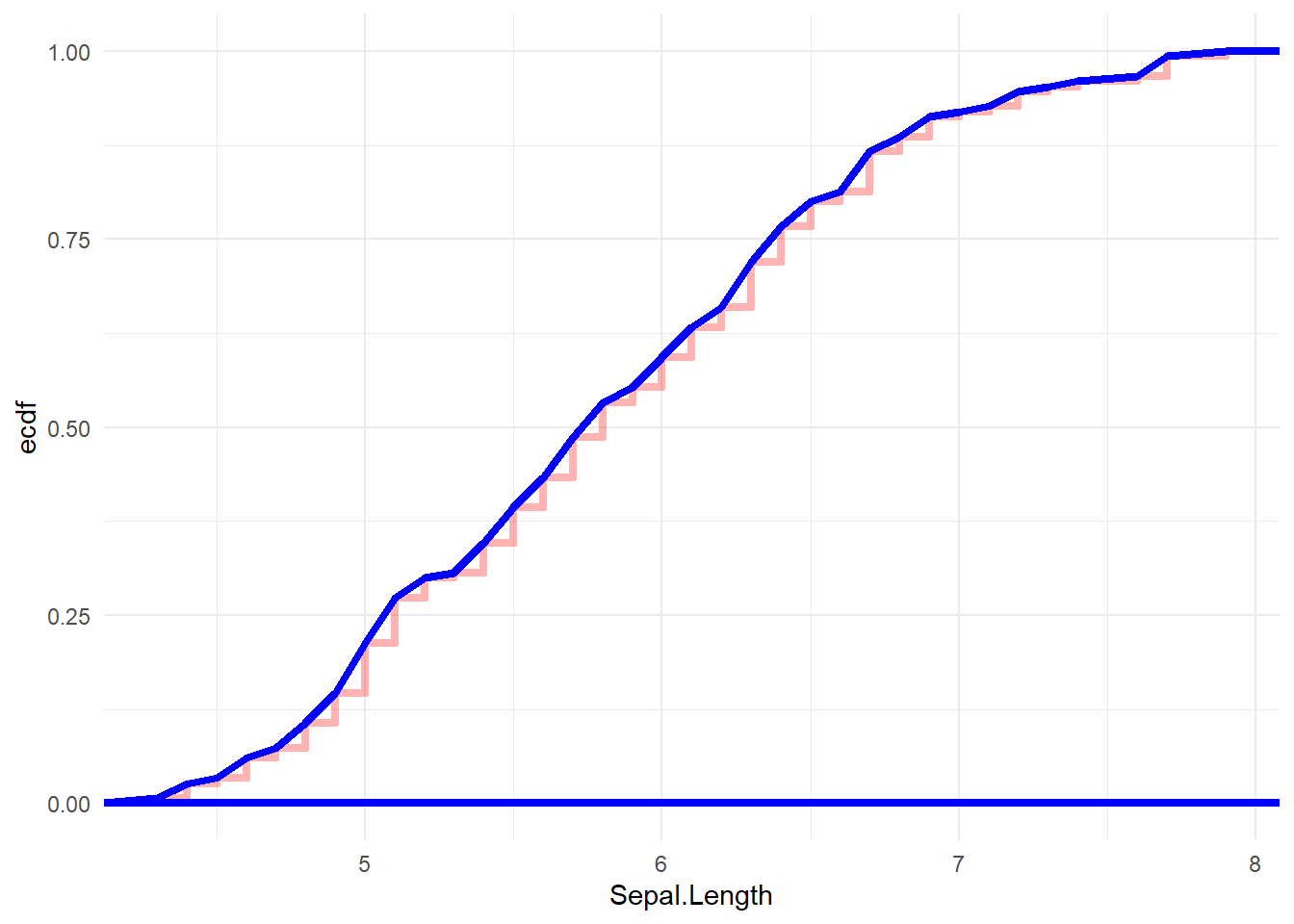
Cumulative Relative Frequency graphs represent the cumulative relative frequency as the values increase (what percentage of values are less than or equal to each x-value). These always range from 0 to 1 on the y-axis (or 0% to 100%).
9.3 Normal Distributions
In the early 19th Century, the mathematicians Gauss and Adrian both noticed that many, many natural processes (like dimensions and weights of plants and animals) and many human processes (manufacturing, scores on tests) follow (approximately, not exactly) a very nice bell-shaped curve that Abraham de Moivre, an 18th century statistician and consultant to gamblers, had developed. This bell-shaped curve is now called the normal curve, and has the equation
\[P(x) = \frac{1}{\sigma\sqrt{2\pi}}e^{\frac{-(x-\mu)^2}{2\sigma^2}}\]
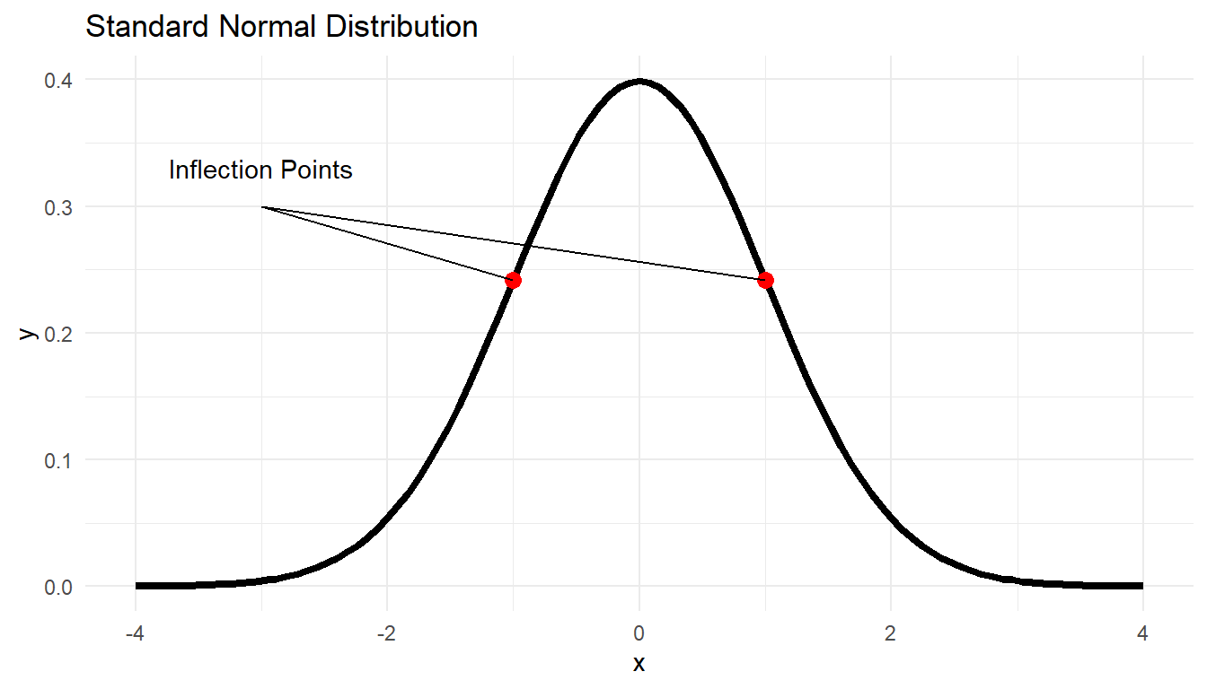
Where \(P(x)\) represents the height of the curve, \(\mu\) is the mean (of all the \(x\)’s), and \(\sigma\) is the standard deviation. If the mean is 0 and the standard deviation is 1, the graph looks like this:

Notice that the inflection points (where the curve changes its concavity, like in a cubic function) are at exactly one standard deviation from the mean, and by the time the graph gets to 3 standard deviationss in each direction, the height of the curve is basically zero.
This is called the Standard Normal Distribution, or \(N(0,1)\). Remember that we use this to approximate real life, and we always need to check that this approximation is appropriate in a given situation.
9.3.1 Characteristics of the Normal Distribution
- They are always unimodal, bell-shaped, and symmetric about the mean
- The x-axis represents different values of the variable, and the probability of any single value of x is zero (not true in real-life situations, but remember that this is an approximation).
- The probability of a range of x-values is shown on the graph by the area under the curve for that range. The shaded area in the Standard Normal graph above represents the probability that \(x\) will be at least 1.5 standard deviations below the mean (about 10%).
- The total area under the curve is 1, or 100%
- The graph can be narrow or broad, depending on the standard deviation, but never skewed.
9.3.2 Empirical Rule
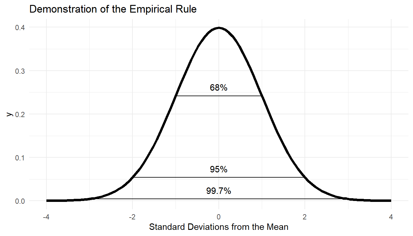
- about 68% of the distribution is within 1 standard deviation of the mean
- about 95% of the distribution is within 2 standard deviation of the mean
- about 99.7% of the distribution is within 3 standard deviation of the mean

9.3.3 Assessing for Normality
When assessing normality, you have to think about what makes a normal distribution…. a normal distribution. Refer to the characteristics of a normal distribution to remind yourself what you need to look for.
- Graph your data using a dot plot, histogram, boxplot, or stem plot. Whichever one is most convenient and would show the distribution of data the best.
- Compare the mean and median of the distribution. Normal curves are symmetric, so our data should also be symmetric. Are the mean and median almost the same?
- Check to see if the data follows the empirical rule. Is there 68% of the data between -1 and 1 standard deviations? What about 95% and 99.7%?
- Look at the normal probability plot if given. (Know how to interpret and read, not make). If the plot is fairly linear (does a straight line fit through the points), then we have further evidence that the distribution is approximately normal
9.3.4 Standardized Score
If \(x\) is an observation that has a known mean and standard deviation, the standardized score of \(x\) is: \[z = \frac{\text{value} - \text{mean}}{\text{standard deviation}}\] A standardized score, often called a z-score, of an observation is the number of standard deviations it is from the mean.
9.3.5 Calculating Probabilities and Percentiles
Using calculus, we could calculate the area (and therefore the probability) under any section of any normal distribution. But we don’t want to have to use calculus every time we want to calculate a normal probability. So, we use a table (inside the front cover of your book and also in Table A) in which many Standard Normal probabilities have been calculated for us. So all we need to do is convert our problem to Standard Normal, and we can use this table. We make this conversion using z-scores.
Once we have a z-score, we can use the Standard Normal table to find a corresponding probability.
9.3.6 Using your Calculator
Remember that to access the calculator functions related to distributions on a TI-83/84 series, you go to:
2nd -> vars (distr)The two functions of interest for this chapter are:
normalcdf(lowerbound, upperbound [, mu, sigma])

invNorm(area to the left of value [, mu, sigma])
When using your calculator to calculate Normal probabilities you need to make sure you write at least the following information to ensure full credit:
- The name of the distribution
- The parameters of the distribution (for normal distributions, the mean and s.d.)
- How to calculate the test statistic (for normal distributions, the z-score)
- The probability you are finding
- The answer in context of the problem
Example
Suppose that the time you need to spend on BART to get from Downtown Berkeley to the SF Airport is approximately normally distributed with \(\mu = 54\) minutes, and \(\sigma = 4.6\) minutes. In other words, BART times from Berkeley to SFO \(\sim N(54, 4.6)\).
Now find each probability (\(X\) represents the amount of time required for a single randomly selected BART trip from Berkeley to SFO):
- \(P(X<53)\) \[ \begin{aligned} z &= \frac{53 - 54}{4.6} \approx -0.22 \\ P(X<53) &\approx P(z < -.22) \underset{\text{Table A}}{=} 0.4129 \end{aligned} \] Using calculator: \[ \begin{aligned} z &= \frac{53 - 54}{4.6} \approx -0.22 \\ P(X<53) &\approx P(z < -0.22) \\ &= \texttt{normalcdf(-1000, -0.22)} \approx 0.4129 \end{aligned} \]
\(P(X>60)\) \[ \begin{aligned} z &= \frac{60 - 54}{4.6} \approx 1.30 \\ P(X>60) &\approx P(z > 1.30) \\ &= 1 - P(z < 1.30) \underset{\text{Table A}}{=} 1 - 0.9032 = 0.0968 \end{aligned} \] Using calculator: \[ \begin{aligned} z &= \frac{60 - 54}{4.6} \approx 1.30 \\ P(X>60) &\approx P(z > 1.30) \\ &= \texttt{normalcdf(1.30, 1000)} \approx 0.0968 \end{aligned} \]
The lowest 5% of travel times are below how many minutes? \[ \begin{aligned} 0.05 & \underset{\text{Table A}}{\approx} P(z<-1.64) \\ \rightarrow z = \frac{x - 54}{4.6} &= -1.64 \\ x &= 46.45 \text{ minutes} \end{aligned} \] Using calculator: \[ \begin{aligned} \texttt{invNorm(0.05)}& \approx P(z<-1.64) \\ \rightarrow z = \frac{x - 54}{4.6} &= -1.64 \\ x &= 46.45 \text{ minutes} \end{aligned} \]